Artificial Neural Network (Part 2): A New Approach of Prediction used in Textiles
Sarita Raut
Lecturer, Sasmira’s Institute of Man Made Textiles, Worli, Mumbai.
sweet_sari2001@yahoo.com
1. Neural Networks Versus Conventional Computers
Neural networks take a different approach to problem solving than that of conventional computers. Conventional computers use an algorithmic approach i.e. the computer follows a set of instructions in order to solve a problem. Unless the specific steps that the computer needs to follow are known the computer cannot solve the problem. That restricts the problem solving capability of conventional computers to problems that we already understand and know how to solve. But computers would be so much more useful if they could do things that we don’t exactly know how to do.
Neural networks process information in a similar way the human brain does. The network is composed of a large number of highly interconnected processing elements (neurons) working in parallel to solve a specific problem. Neural networks learn by example. They cannot be programmed to perform a specific task. The examples must be selected carefully otherwise useful time is wasted or even worse the network might be functioning incorrectly. The disadvantage is that because the network finds out how to solve the problem by itself, its operation can be unpredictable.
On the other hand, conventional computers use a cognitive approach to problem solving; the way the problem is to solved must be known and stated in small unambiguous instructions. These instructions are then converted to a high level language program and then into machine code that the computer can understand. These machines are totally predictable; if anything goes wrong is due to a software or hardware fault.
Neural networks and conventional algorithmic computers are not in competition but complement each other. There are tasks are more suited to an algorithmic approach like arithmetic operations and tasks that are more suited to neural networks. Even more, a large number of tasks, require systems that use a combination of the two approaches (normally a conventional computer is used to supervise the neural network) in order to perform at maximum efficiency.
1.1 Human and Artificial Neurons
1.1.1 How the Human Brain Learns?
Much is still unknown about how the brain trains itself to process information, so theories abound. In the human brain, a typical neuron collects signals from others through a host of fine structures called dendrites. The neuron sends out spikes of electrical activity through a long, thin stand known as an axon, which splits into thousands of branches. At the end of each branch, a structure called a synapse converts the activity from the axon into electrical effects that inhibit or excite activity from the axon into electrical effects that inhibit or excite activity in the connected neurons. When a neuron receives excitatory input that is sufficiently large compared with its inhibitory input, it sends a spike of electrical activity down its axon. Learning occurs by changing the effectiveness of the synapses so that the influence of one neuron on another changes.
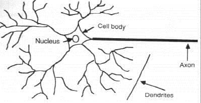
Fig. No. 1 – Components of a neuron
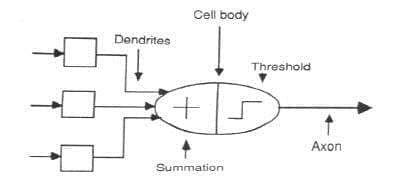
1.1.2 From Human Neurons to Artificial Neurons
We conduct these neural networks by first trying to deduce the essential features of neurons and their interconnections. We then typically program a computer to simulate these features. However because our knowledge of neurons is incomplete and our computing power is limited, our models are necessarily gross idealizations of real networks of neurons.
- Network Properties
The topology of a neural network refers to its framework as well as its interconnection scheme. The framework id often specified by the number of layers and the number of nodes per layer or network layer.
Network layers
The commonest type of artificial neural network consists of three groups, or layers, of units: a layer of “input” units is connected to a layer of “hidden” units, which is connected to a layer of “output” units.
- The input layer: the nodes in it are called input units, which encode the instance presented to the network for processing. The activity of the input units represents the raw information that is fed into the network.
- The hidden layer: the nodes in it are called hidden units, which are not directly observable and hence hidden. They provide nonlinearities for the network. The activity of each hidden unit is determined by the activities of the input units and the weights on the connections between the input and the hidden units.
- The output layer: the nodes in it are called output units, which encode possible concepts to be assigned to the instance under consideration. The behavior of the output units depends on the activity of the hidden units and the weights between the hidden and output units.
This simple type of network is interesting because the hidden units are free to construct their own representations of the input. The weights between the input and hidden units determine when each hidden unit is active, and so by modifying these weights, a hidden unit can choose what it represents [1,2]
3. Architecture of Neural Networks
3.1 Feed-forward networks
Feed-forward ANNs (figure 3.5) allow signals to travel one way only; from input to output. There is no feedback (loops) i.e. the output of any layer does not affect that same layer. Feed-forward ANNs tend to be straight forward networks that associate inputs with outputs. They are extensively used in pattern recognition

Fig. No. 3 – Simple feedforward Neural network with two inputs, two hidden layers and one output.
3.2 Feedback networks
Feedback networks can have signals travelling in both directions by introducing loops in the network. Feedback networks are very powerful and can get extremely complicated. Feedback networks are dynamic; their ‘state’ is changing continuously until they reach an equilibrium point. They remain at the equilibrium point until the input changes and a new equilibrium needs to be found.
3.3 The Learning Process
Learning Rules:-We define a learning rule as a procedure for modifying the weights and biases of a network. (This procedure may also be referred to as a training algorithm.) The learning rule is applied to train the network to perform some particular task. Learning rules in this toolbox fall into two broad categories: supervised learning, and unsupervised learning.
All learning methods used for adaptive neural networks can be classified into two major categories:
Supervised learning [45] which incorporates an external teacher, so that each output unit is told what its desired response to input signals ought to be. Supervised learning is a machine learning technique for creating a function from training data. In supervised learning, the learning rule is provided with a set of examples (the training set) of proper network behavior. As the inputs are applied to the network, the network outputs are compared to the targets. The learning rule is then used to adjust the weights and biases of the network in order to move the network outputs closer to the targets. The perceptron learning rule falls in this supervised learning category.
The training data consist of pairs of input objects (typically vectors), and desired outputs. The output of the function can be a continuous value (called regression), or can predict a class label of the input object (called classification). The task of the supervised learner is to predict the value of the function for any valid input object after having seen a number of training examples (i.e. pairs of input and target output). To achieve this, the learner has to generalize from the presented data to unseen situations in a “reasonable” way (see inductive bias). (Compare with unsupervised learning.) The parallel task in human and animal psychology is often referred to as concept learning .
During the learning process global information may be required. Paradigms of supervised learning include error-correction learning, reinforcement learning and stochastic learning.
An important issue concerning supervised learning is the problem of error convergence, i.e. the minimization of error between the desired and computed unit values. The aim is to determine a set of weights which minimizes the error. One well-known method, which is common to many learning paradigms is the least mean square (LMS) convergence.
Unsupervised learning uses no external teacher and is based upon only local information. It is also referred to as self-organizing . In unsupervised learning, the weights and biases are modified in response to network inputs only. There are no target outputs available. Most of these algorithms perform clustering operations. They categorize the input patterns into a finite number of classes. This is especially useful in such applications as vector quantization
Learning Rates:-The rate at which ANNs learn depends upon several controllable factors. In selecting the approach there are many trade-offs to consider. Obviously, a slower rate means a lot more time is spent in accomplishing the off-line learning to produce an adequately trained system. With the faster learning rates, however, the network may not be able to make the fine discriminations possible with a system that learns more slowly. Researchers are working on producing the best of both worlds.
3.4 Transfer Function
The behavior of an ANN (Artificial Neural Network) [3]depends on both the weights and the input-output function (transfer function) that is specified for the units. This transfer function is commonly used in back propagation networks. This function typically falls into one of three categories. Three of the most commonly used functions are shown below.
1. The hard-limit transfer function:- As shown in the fig. limits the output of the neuron to either 0, if the net input argument n is less than 0, or 1, if n is greater than or equal to 0. This function is used in Perceptions, to create neurons that
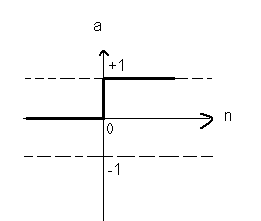
make classification decisions.
a= hardlim(n)
Fig. No. 4 – Hard-limit transfer function
- Linear transfer function:- As shown in the fig. below the neurons of this type are used as linear approximators in Linear Filters.
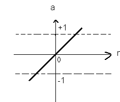
a= purelin(n)
Fig. No. 5. Linear transfer function
- Sigmoid transfer function : As shown figure below , it takes the input, which can have any value between plus and minus infinity, and squashes the output into the range 0 to 1.
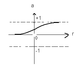
a= logsin(n)
Fig. No. 6 – Log-Sigmoid transfer function
3.5 The Back-Propagation Algorithm
Multilayer network can be trained using various algorithms, although the method called “Back-Propagation” is the most widely used. Back-Propagation is a powerful, flexible training algorithm, though training speed is slow.
The back-propagation learning algorithm was proposed by rumelhart et al. in 1986 to modify connection weight in multilayered feed forward networks. The back-propagation algorithm is an iterative gradient descent algorithm that minimizes the sum of the squared error between the desired output and actual output [4].
Backpropagation was created by generalizing the Widrow-Hoff learning rule to multiple-layer networks and nonlinear differentiable transfer functions. Input vectors and the corresponding target vectors are used to train a network until it can approximate a function, associate input vectors with specific output vectors, or classify input vectors in an appropriate way as defined by you. Networks with biases, a sigmoid layer, and a linear output layer are capable of approximating any function with a finite number of discontinuities.
Standard backpropagation is a gradient descent algorithm, as is the Widrow-Hoff learning rule, in which the network weights are moved along the negative of the gradient of the performance function. The term backpropagation refers to the manner in which the gradient is computed for nonlinear multilayer networks. There are a number of variations on the basic algorithm that are based on other standard optimization techniques, such as conjugate gradient and Newton methods.
Properly trained backpropagation networks tend to give reasonable answers when presented with inputs that they have never seen. Typically, a new input leads to an output similar to the correct output for input vectors used in training that are similar to the new input being presented. This generalization property makes it possible to train a network on a representative set of input/target pairs and get good results without training the network on all possible input/output pairs. There are two features of the Neural Network Toolbox that are designed to improve network generalization – regularization and early stopping.
3.6 Applications of Neural Networks
Neural networks have broad applicability to real world business problems. In fact, they have already been successfully applied in many industries. Since neural networks are best at identifying patterns or trends in data, they are well suited for prediction or forecasting needs including:
Sales forecasting
Industrial process control
Customer research
Data validation
Risk management
Target marketing
But to give you some more specific examples; ANN are also used in the specific paradigms: such as:
- Recognition of speakers in communications;
- Diagnosis of hepatitis;
- Recovery of telecommunications from faulty software;
- Interpretation of multimeaning Chinese words;
- Undersea mine detection;
- Texture analysis;
- Three-dimensional object recognition;
- Hand-written word recognition;
- Facial recognition.
Basically, most applications of NN in textiles fall into five categories: Prediction, classification, data association, data conceptualization and data filtering.
- Prediction: refers to predicting some output from inputs using ANN. E.g. predication of tensile properties.
- Classification: used to identify an unknown pattern that exists in a data.
- Data association: refers to recognizing data that contains error. It can be used both for identifying the characters that were scanned and also for identifying scanner when it is not working properly.
- Data conceptualization: it is inferring grouping relationships from the input data. (System modeling, Synthesis etc).
- Data filtering: it is concerned with the smoothening of input data. It can also be used for taking away noise from the input data. [1].
References:
- Rajamanikam, R., Hansen, Jayaraman, “Analysis of modeling methodologies for predicting the strength of air jet spun yarn”, Textile Res. J. 67(1), 39-44 (1997)
- Zaman R. and Wunsch, C.” Prediction of yarn strength from fibre properties from fuzzy ARTMAP, 1997.
https://www.acil.ttu.edu/users/Raonak/papers/itc.htm.
- Introduction to MATLAB for Engineers and Scientists, Belores M. Etter.
- Chattopadhyay, R., and Guha, A., “Artificial Neural Networks: Applications to Textile”, The Textile Institute, Manchester, Textile Progress 2004.